Resources
Highlights
Summary
This project implements CellMap, a community-driven mobile network mapping platform designed to collect, process, and map crowd-sourced mobile network measurements across Italy.
Main actors and features
The system is designed around three main categories of users:
- Regular users: Can run internet speed-tests (measuring download, upload, and latency metrics) and open configuration tickets when they detect unmapped or broken cells
- Administrators: They process a sequential queue of tickets to approve, modify, or discard proposed infrastructure modifications
- Host users (ISPs): Participate in the platform by hosting speed-test servers to route regular users’ connection requests
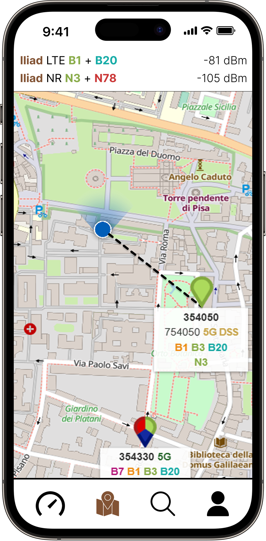
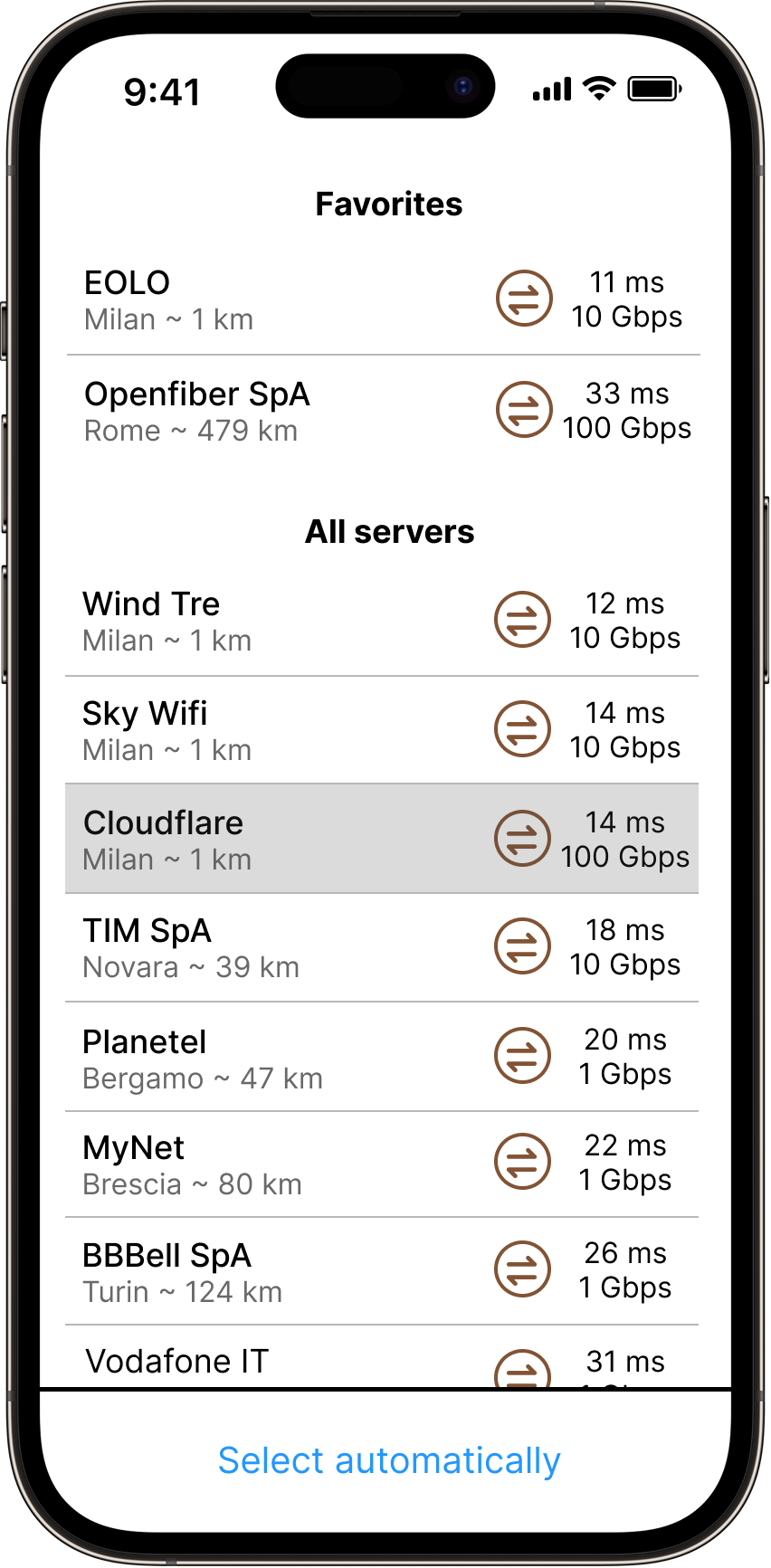
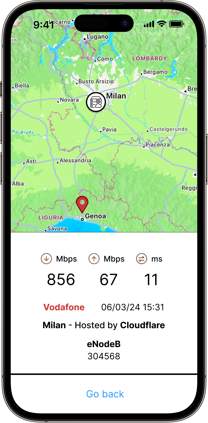
Regular users can search for a location in Italy to identify the closest antennas, view detailed node characteristics (operating frequencies, 5G status), check average speeds achieved in that area, and compare performance by mobile carrier.
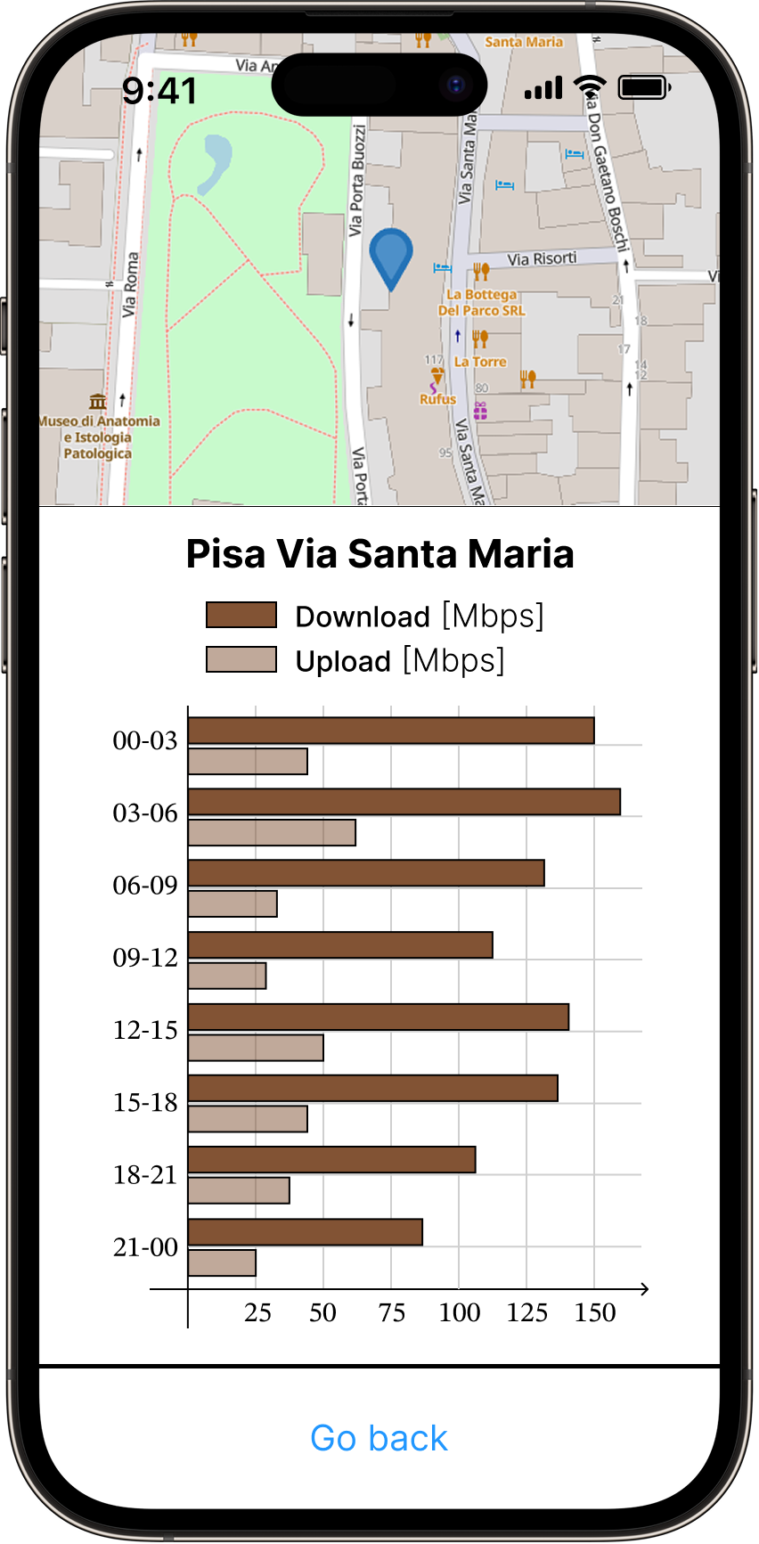
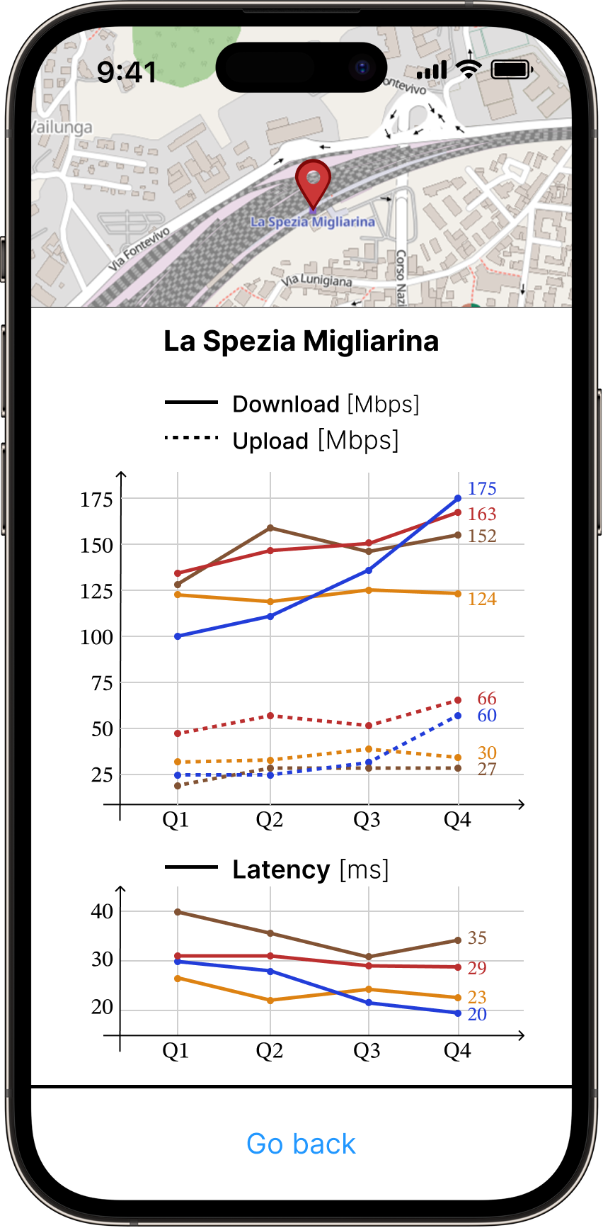
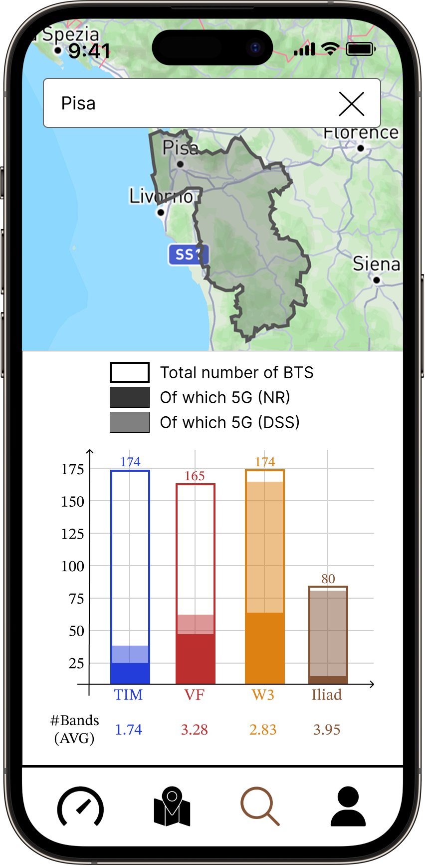
User Interface Mock-ups
Distributed architecture
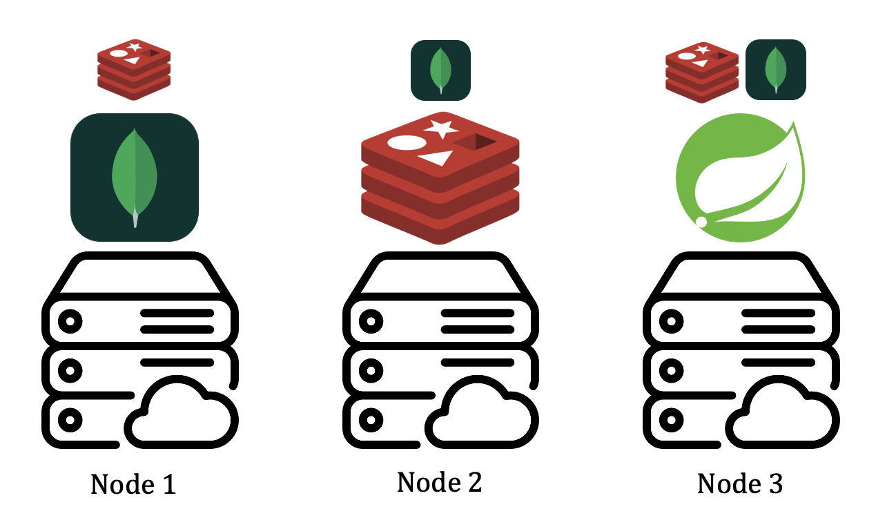
To achieve high availability and load distribution, the software stack is distributed across a 3-node cluster:
- Node 1: Serves as the MongoDB primary node, while also hosting a Redis replica instance and a Redis Sentinel instance to participate in automated failover orchestration
- Node 2: Serves as the Redis master node. Simultaneously, it hosts a MongoDB secondary instance and the second Redis Sentinel instance
- Node 3: Hosts the Spring Boot REST API backend application. To optimize data retrieval performance, it also hosts a MongoDB secondary replica and a Redis replica plus Sentinel instance. This allows the local Spring Boot application to leverage the
nearestread preference, fetching data directly from the local host memory
Database design
Database design
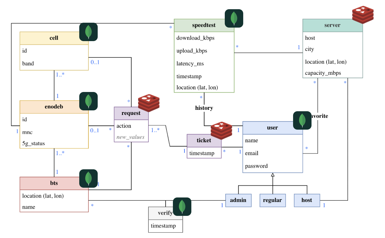
The system separates concerns between MongoDB for long-term storage and analytical queries, and Redis for low-latency, volatile, and simple access patterns:
MongoDB collections
users: Stores user credentials and accounts. It contains afavorite_serversarray storing only numeric server IDs to avoid duplicating server details which reside in Redisspeedtests: A flat collection containing download/upload speeds, latency, timestamps, and GeoJSON locationsbts: Employs an embedded hierarchy to represent physical towers:BTS\(\rightarrow\)eNodeB\(\rightarrow\)Cell. Since the number of cells/eNodeBs per tower is small and stable, embedding them prevents unnecessary joins and keeps reads highly efficient
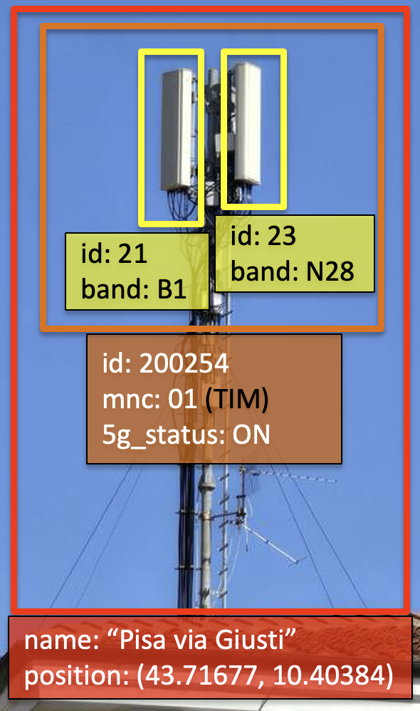
Redis Key Structure
- Servers: The list of speedtest servers is stored in Redis because it is queried constantly but rarely changes
servers:active: A Sorted Set populated usingGEOADDfor low-latency coordinates-based geospatial queriesservers:id_counter: A String counter used to auto-increment server IDsserver:<id>: A Hash storing server details (host, city, capacity, etc.)
- Tickets & Requests (Redis Streams):
Instead of a naive key-value approach (such as storing
ticket:<id>:timestampandticket:<id>:<request_id>), tickets and requests are managed via a singleticketskey of type STREAM. Redis Streams act as append-only logs supporting consumer group patterns (adminsgroup):- 1 RTT query execution to claim the oldest pending ticket
- Thread-safety by default when multiple administrators handle tickets
- Automatic ticket ID management via the stream’s entry IDs
Main queries
Query i
Given an eNodeB (MNC + node ID) and a timestamp, this query computes the median download, upload, and latency metrics alongside the total test count, aggregated by three-hour time slots
db.speedtests.aggregate([
  // Stage 1: Filter the speed-tests by node and timestamp
  { $match: { enodeb: enodeb, mnc: mnc, timestamp: { $gte: timestamp } } },
  // Stage 2: Group the filtered speed-tests by three-hour time slots and compute median metrics
  {
    $group: {
      _id: {
        $hour: { $dateTrunc: { date: "$timestamp", unit: "hour", binSize: 3 } }
      },
      number_of_tests: { $sum: 1 },
      median_download_kbps: { $median: { input: "$download_kbps", method: "approximate" } },
      median_upload_kbps: { $median: { input: "$upload_kbps", method: "approximate" } },
      median_latency_ms: { $median: { input: "$latency_ms", method: "approximate" } }
    }
  }
]);
Query ii
Given a location \(L\) (latitude, longitude) and a radius \(R\) (meters), this query computes the median metrics per carrier recorded within the radius during the last four complete trimesters
db.speedtests.aggregate([
  // Stage 1: Filter speed-tests within the specified region
  {
    $geoNear: {
      near: { type: "Point", coordinates: [lon, lat] },
      distanceField: "distance_from_L_meters",
      maxDistance: radius,
      spherical: true
    }
  },
  // Stage 2: Keep only speed-tests from the last four complete trimesters
  {
    $addFields: {
      start_of_current_quarter: { $dateTrunc: { date: "$$NOW", unit: "quarter" } }
    }
  },
  {
    $match: {
      $expr: {
        $and: [
          { $lt: [ "$timestamp", "$start_of_current_quarter" ] },
          { $gte: [ "$timestamp", { $dateSubtract: { startDate: "$start_of_current_quarter", unit: "year", amount: 1 } } ] }
        ]
      }
    }
  },
  // Stage 3: Add the year and month fields to identify the trimester
  {
    $addFields: {
      year: { $year: "$timestamp" },
      month: { $dateTrunc: { date: "$timestamp", unit: "quarter" } }
    }
  },
  // Stage 4: Group by carrier and trimester, computing the median values
  {
    $group: {
      _id: { mnc: "$mnc", year: "$year", month: "$month" },
      number_of_tests: { $sum: 1 },
      median_download_kbps: { $median: { input: "$download_kbps", method: "approximate" } },
      median_upload_kbps: { $median: { input: "$upload_kbps", method: "approximate" } },
      median_latency_ms: { $median: { input: "$latency_ms", method: "approximate" } }
    }
  }
]);
Query iii
Given a province (e.g. "PI" for Pisa), this query calculates the total number of physical towers per carrier, the percentage of 5G towers (both DSS and NR), and the average number of bands per tower
db.bts.aggregate([
  // Stage 1: Filter the BTS and unwind the nodes array
  { $match: { province: province } },
  { $unwind: "$nodes" },
  // Stage 2: Compute BTS-specific results for each carrier
  {
    $group: {
      _id: { bts_id: "$_id", mnc: "$nodes.mnc" },
      has_5g_nr: { $max: { $cond: [{ $eq: ["$nodes.5g_status", "YES"] }, 1, 0] } },
      has_5g_dss: { $max: { $cond: [{ $eq: ["$nodes.5g_status", "DSS"] }, 1, 0] } },
      nested_bands: { $push: "$nodes.cells.band" }
    }
  },
  // Count the unique bands
  {
    $addFields: {
      unique_bands_count: {
        $size: {
          $reduce: {
            input: "$nested_bands",
            initialValue: [],
            in: { $setUnion: ["$$value", "$$this"] }
          }
        }
      }
    }
  },
  // Stage 3: Group by carrier to compute the final statistics
  {
    $group: {
      _id: "$_id.mnc",
      bts_count: { $sum: 1 },
      bts_with_5g_nr_percent: { $avg: { $cond: ["$has_5g_nr", 100, 0] } },
      bts_with_5g_dss_percent: { $avg: { $cond: ["$has_5g_dss", 100, 0] } },
      avg_bands_per_bts: { $avg: "$unique_bands_count" }
    }
  }
]);
Query iv
Find the \(N\) closest active servers to a user’s location
# Step 1: Fetch the IDs of nearby servers
GEORADIUS servers:active <lon> <lat> 500 km ASC COUNT N WITHDIST

# Step 2: Fetch the details of the returned IDs (pipelined)
HGETALL server:<id>
Query v
Producers (users) append modification proposals, and consumers (administrators) sequentially claim and resolve them
# Setup the consumer group and stream
XGROUP CREATE tickets admins $ MKSTREAM

# User submits a ticket with an embedded requests array
XADD tickets * user '{"_id": "68a785e9b5bcf321922694e4", "name": "antirez"}' requests '[{"action": "MOVE_BTS", "bts": "68a78cd88742bc1b450e62bc", "lat": 45.467, "lon": 9.19}]'

# Admin claims the oldest pending ticket not yet assigned
XREADGROUP GROUP admins <admin_name> COUNT 1 STREAMS tickets >

# Admin acknowledges and removes the processed ticket from the stream
XACKDEL tickets admins <id>
Database replication
The system prioritizes availability and partition tolerance (AP paradigm in the CAP theorem) by defining replication parameters and future sharding rules:
Replication settings
- MongoDB write concern:
{w: 1, j: false}forspeedteststo maximize ingestion speed (occasional loss of a speedtest is acceptable),{w: "majority", j: false}elsewhere
- Redis configuration:
- RAM utilization is low (\(< 1\) MB), so the default
noevictionpolicy is used - Snapshotting is scheduled every 10 minutes (
save 600 1) instead of writing Append-Only Files (AOF) to eliminate I/O write overhead
- RAM utilization is low (\(< 1\) MB), so the default
Future sharding plans
As data volumes grow, sharding can be introduced as follows:
users: Shard by_idto distribute accounts evenlybts: Shard byprovince. This ensures all towers in the same province reside on the same shard, keeping provincial comparison queries localspeedtests: Shard using geohashing on the GeoJSON location. This guarantees geographically close speed tests are co-located on the same shard, preserving the efficiency of spatial queries
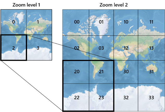
Geohashing
Performance optimization
Finally, targeted secondary and geospatial indexes were configured in MongoDB:
speedtests.enodeb: Speeds up the hourly eNodeB performance analytics query. The index reduces execution times from 283 ms to 4 msbts.province: Optimizes carrier-comparison analytics by province, dropping execution times from 86 ms to 11 msbts.nodes.id: Allows the API to instantly verify cell existence in the database (e.g., when a user connects to a new cell). The index drops lookup times from 80 ms to 0 ms- Geospatial Indexes:
2dsphereindexes onbts.locationandspeedtests.locationare used to run$geoNearaggregation queries